Financial Model - Phase 2: Calculations Engine
Build the 12-month projection model with formulas
Financial Model - Phase 2: Calculations Engine
Welcome back! In Phase 1, you built the inputs. Now you'll build the calculation engine.
Phase Progress
✅ Phase 1: Setup & Inputs (Complete!) 🔵 Phase 2: Calculations Engine (You are here)
- Phase 3: Analysis & Metrics
- Phase 4: Dashboard & Polish
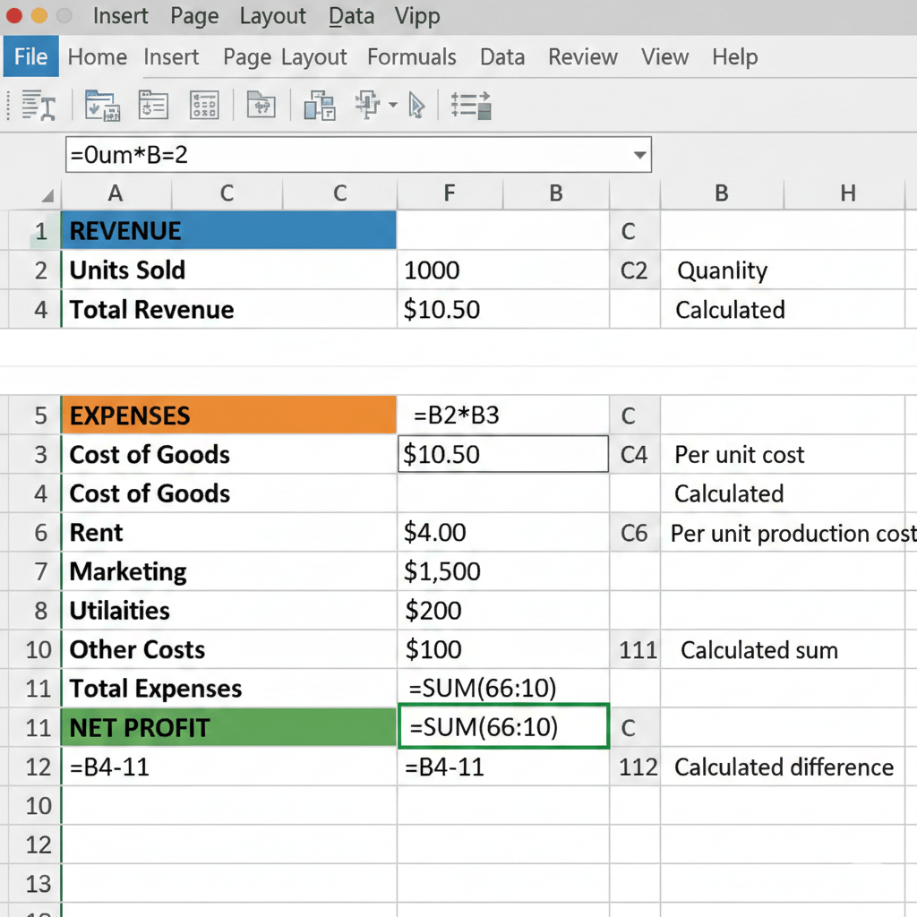
Step 3: Create the Calculations Sheet Structure
Now we build the engine that does all the math.
Why this matters: This is where Excel's power shows. You'll enter formulas once, and they'll calculate for all 12 months automatically.
Instructions:
- Click the Calculations tab
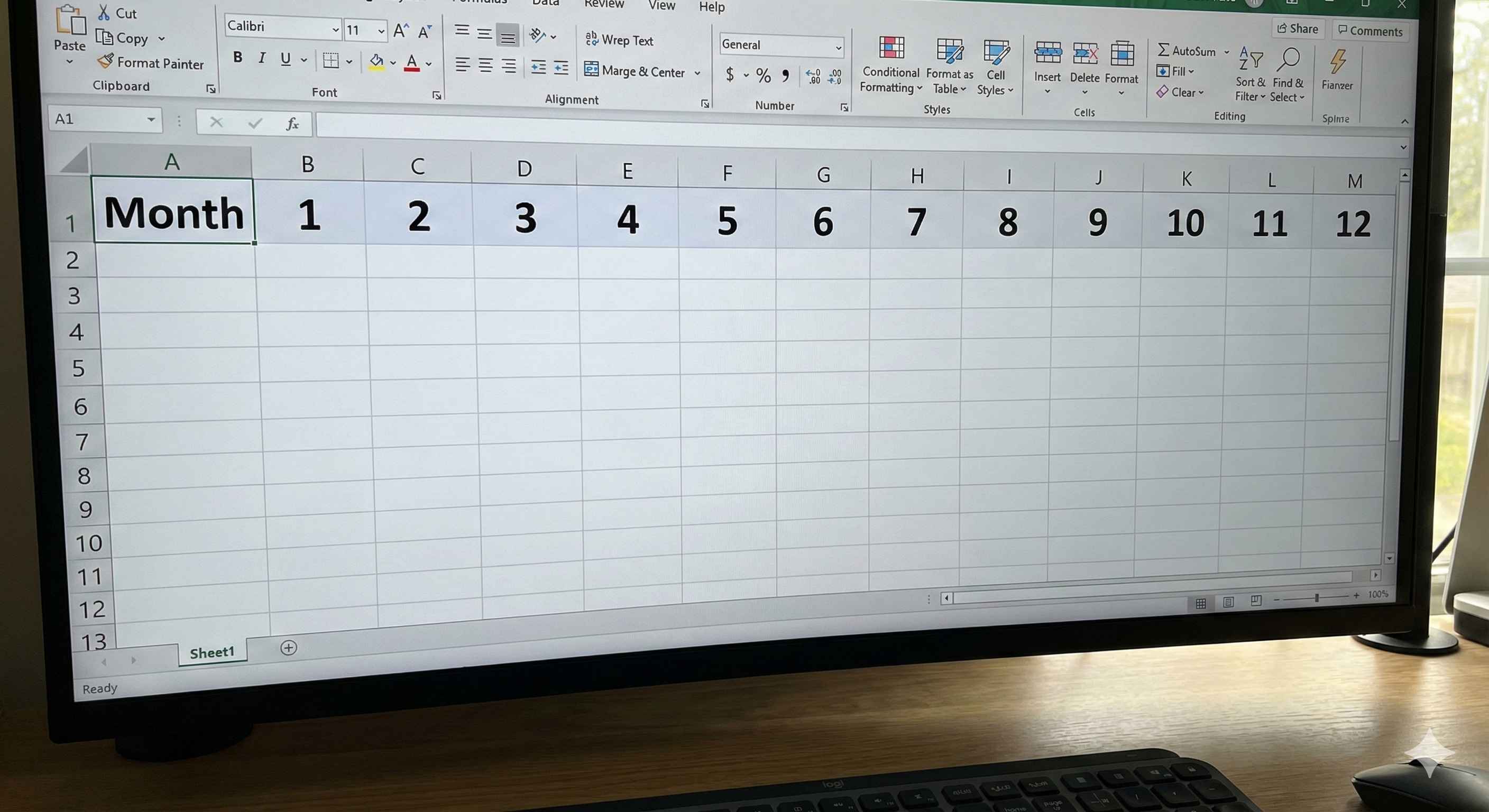
- Build the header row:
| Cell | Type This |
|---|---|
| A1 | Month |
| B1 | 1 |
| C1 | 2 |
| D1 | 3 |
| E1 | (continue to M1 = 12) |
Quick way to fill 1-12:
- Type 1 in B1, type 2 in C1
- Select B1:C1
- Grab the fill handle (small square bottom-right)
- Drag right to M1
- Excel fills 3, 4, 5... 12 automatically!
- Add row labels in column A:
| Cell | Type This | What it means |
|---|---|---|
| A3 | REVENUE | Section header |
| A4 | Units Sold | Quantity sold |
| A5 | Price per Unit | Selling price |
| A6 | Total Revenue | Units × Price |
| A8 | EXPENSES | Section header |
| A9 | Cost of Goods | Ingredient costs |
| A10 | Rent | Monthly rent |
| A11 | Marketing | Monthly marketing |
| A12 | Utilities | Monthly utilities |
| A13 | Other Costs | Monthly other |
| A14 | Total Expenses | Sum of all expenses |
| A16 | NET PROFIT | Revenue - Expenses |
- Format the section headers:
- Select A3, make it Bold + Blue background
- Select A8, make it Bold + Orange background
- Select A16, make it Bold + Green background
✓ Checkpoint: You should have:
- Months 1-12 across the top (B1:M1)
- Revenue section (rows 3-6)
- Expenses section (rows 8-14)
- Net Profit row (row 16)
Step 4: Write Revenue Formulas (The Growth Engine)
Now the magic happens. We'll create formulas that reference the Inputs sheet.
Why this matters: When you change a price on the Inputs sheet, all 12 months update instantly. This is the power of Excel.
Instructions:
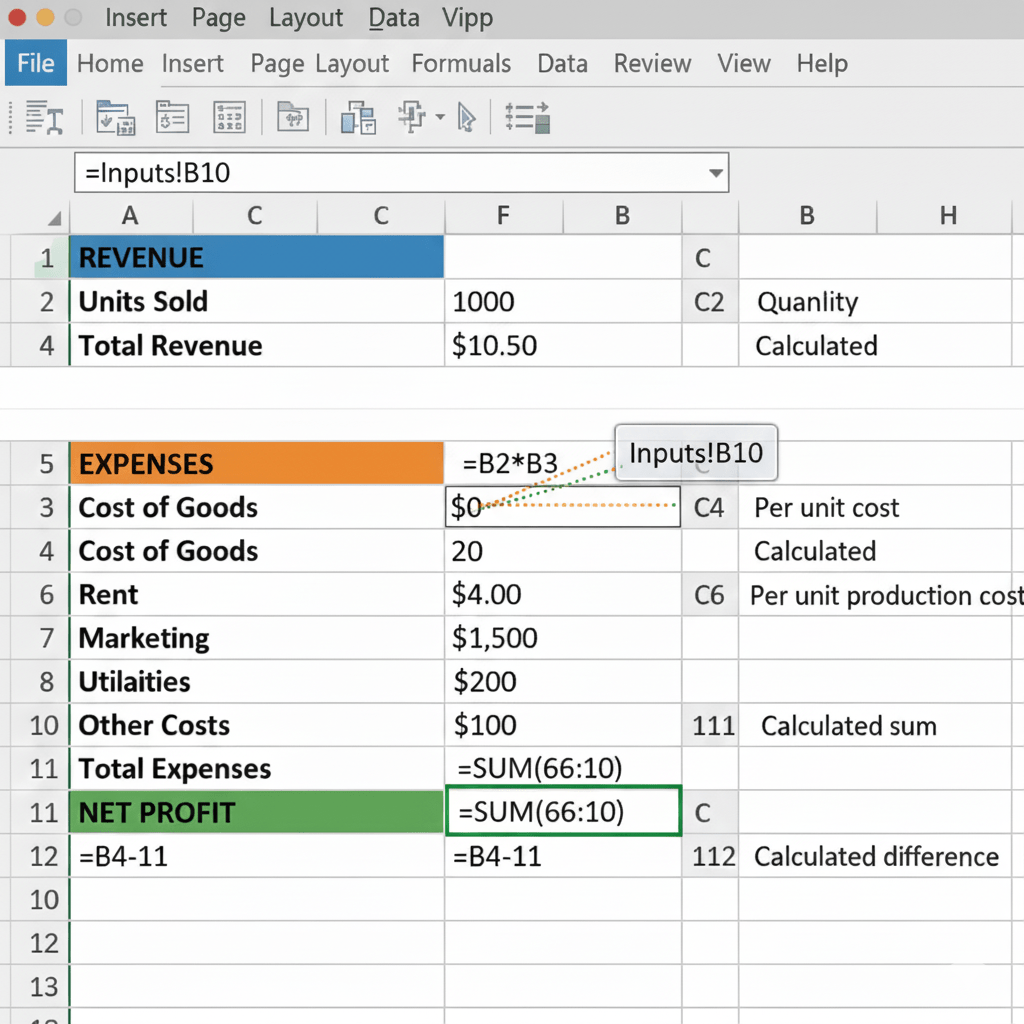
- Calculate Units Sold for Month 1:
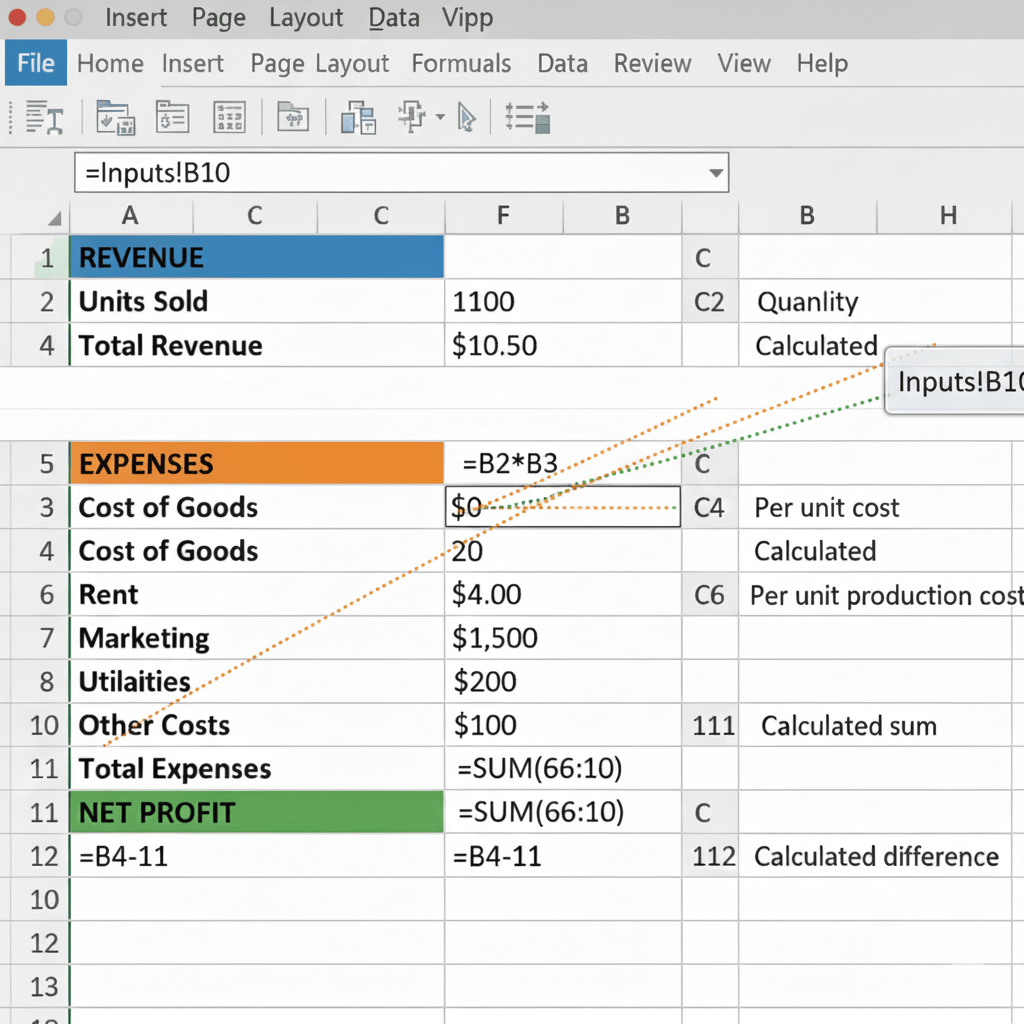
- Click cell B4 (Units Sold, Month 1)
- Type:
=Inputs!B10 - Press Enter
- You should see: 20
What this means: The = sign starts a formula. Inputs!B10 means "go to the Inputs sheet, get the value from cell B10"
- Calculate Units Sold for Month 2 (with growth):
- Click cell C4 (Units Sold, Month 2)
- Type:
=B4*(1+Inputs!$B$11) - Press Enter
- You should see: 22 (20 + 10% growth)
Breaking down the formula:
B4= Previous month's units (20)*= Multiply(1+Inputs!$B$11)= (1 + 10%) = 1.10- Result: 20 × 1.10 = 22
The $ signs lock the growth rate reference so it doesn't change when we copy.
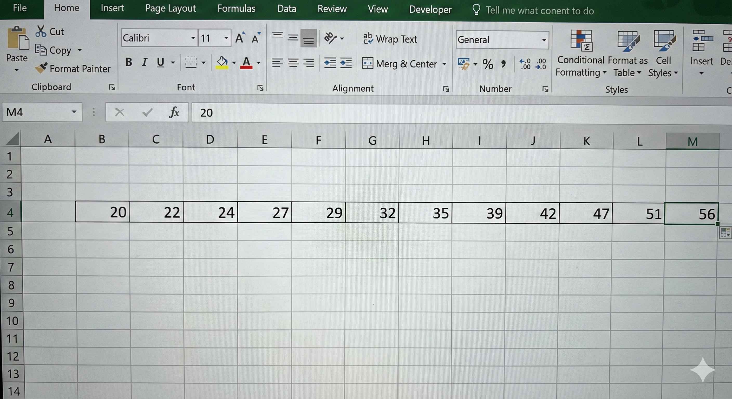
- Copy the growth formula across all months:
- Select cell C4
- Copy the formula right to M4 (drag the fill handle)
- You should see units growing each month: 22, 24, 27, 29...
-
Add Price per Unit (stays constant):
- Click cell B5
- Type:
=Inputs!$B$9 - Press Enter (shows $50)
- Copy this formula right to M5 (drag fill handle)
- All months show $50
-
Calculate Total Revenue:
- Click cell B6
- Type:
=B4*B5 - Press Enter (shows $1,000)
- Copy right to M6
✓ Checkpoint: Row 6 should show revenue growing each month:
- Month 1: $1,000
- Month 2: $1,100
- Month 3: $1,210
- Month 12: around $3,138
Step 5: Calculate Expenses (The Cost Side)
Expenses are simpler - most stay the same each month.
Instructions:
- Calculate Cost of Goods (variable cost):
- Click B9 (Cost of Goods, Month 1)
- Type:
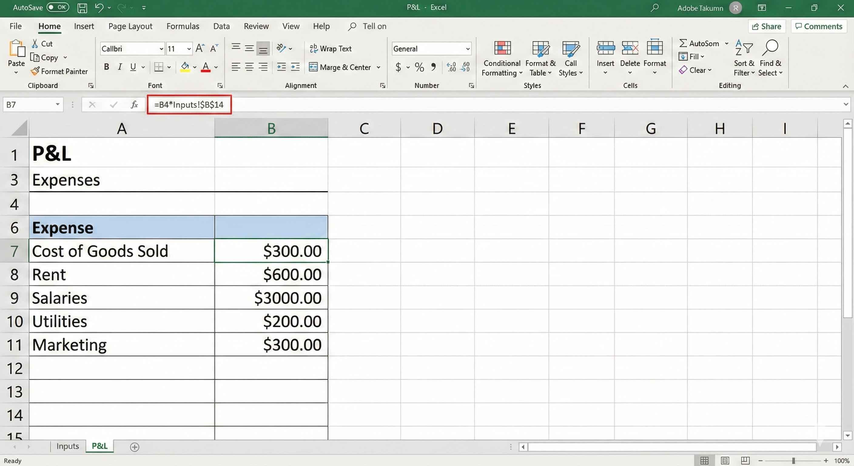
=B4*Inputs!$B$14 - Press Enter (shows $300)
- What this does: Units Sold (20) × Cost per Unit ($15) = $300
- Copy right to M9
-
Add Fixed Expenses (same every month):
- Click B10 (Rent)
- Type:
=Inputs!$B$15 - Press Enter (shows $500)
- Copy right to M10
-
Repeat for other fixed costs:
| Row | Cell | Formula | Result |
|---|---|---|---|
| Marketing | B11 | =Inputs!$B$16 | $200 |
| Utilities | B12 | =Inputs!$B$17 | $100 |
| Other Costs | B13 | =Inputs!$B$18 | $150 |
Copy each formula across to column M (month 12).
- Calculate Total Expenses:
- Click B14
- Type:
=SUM(B9:B13) - Press Enter (shows $1,250)
- Copy right to M14
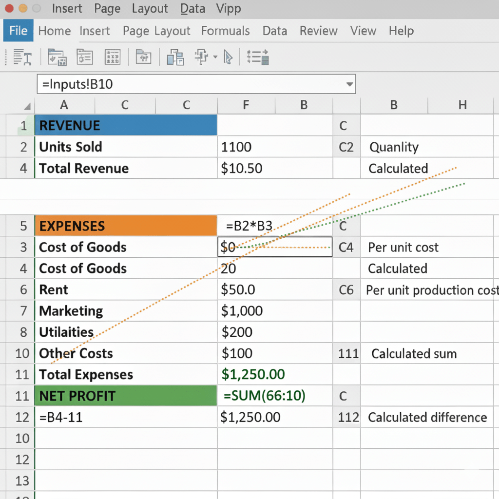
✓ Checkpoint: Month 1 expenses should be:
- Cost of Goods: $300
- Rent: $500
- Marketing: $200
- Utilities: $100
- Other: $150
- Total: $1,250
Step 6: Calculate Net Profit (The Bottom Line)
The moment of truth - are we making money?
Instructions:
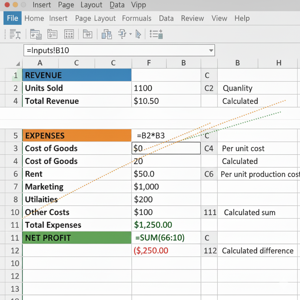
- Click cell B16 (Net Profit, Month 1)
- Type:
=B6-B14 - Press Enter
- You should see: -$250 (negative = loss)
This means: In month 1, we lose $250 because expenses ($1,250) are more than revenue ($1,000).
- Copy the formula right to M16
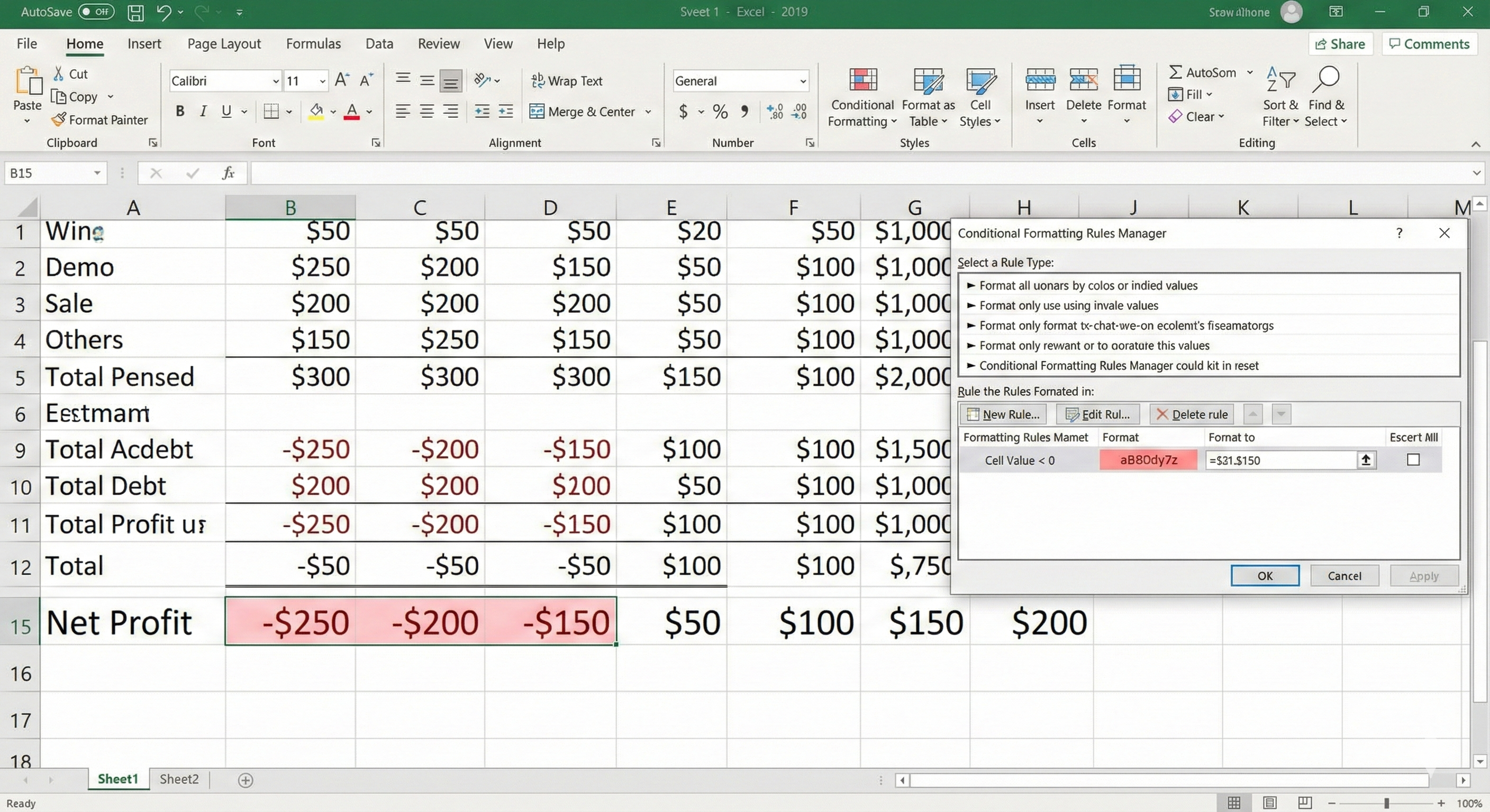
- Add conditional formatting to highlight losses:
- Select B16:M16 (all profit cells)
- Home tab → Conditional Formatting → Highlight Cell Rules → Less Than
- Type: 0
- Choose: Light Red Fill
- Click OK
Now negative months show in red!
✓ Checkpoint: You should see:
- Month 1: -$250 (red, we're losing money)
- Month 2: -$200 (red)
- Around month 4-5: Profit turns positive (no red)
- Month 12: Profit around $1,788