PivotTables
Summarize thousands of rows in seconds
PivotTables
PivotTables are Excel's most powerful feature. They summarize large amounts of data in seconds.
The Problem PivotTables Solve
Imagine you have 1000 rows of sales data. Each row has: Date, Product, Salesperson, Amount.
You want to know: How much did each product sell?
Without PivotTable: Write formulas, filter, copy, paste. Takes 30 minutes.
With PivotTable: Drag and drop. Takes 30 seconds.
What a PivotTable Does
A PivotTable takes your raw data and creates summaries automatically.
Your raw data (1000 rows):
| Date | Product | Salesperson | Amount |
|---|---|---|---|
| Jan 1 | Laptop | John | 1000 |
| Jan 2 | Mouse | Mary | 25 |
| Jan 3 | Laptop | John | 1000 |
| ... | ... | ... | ... |
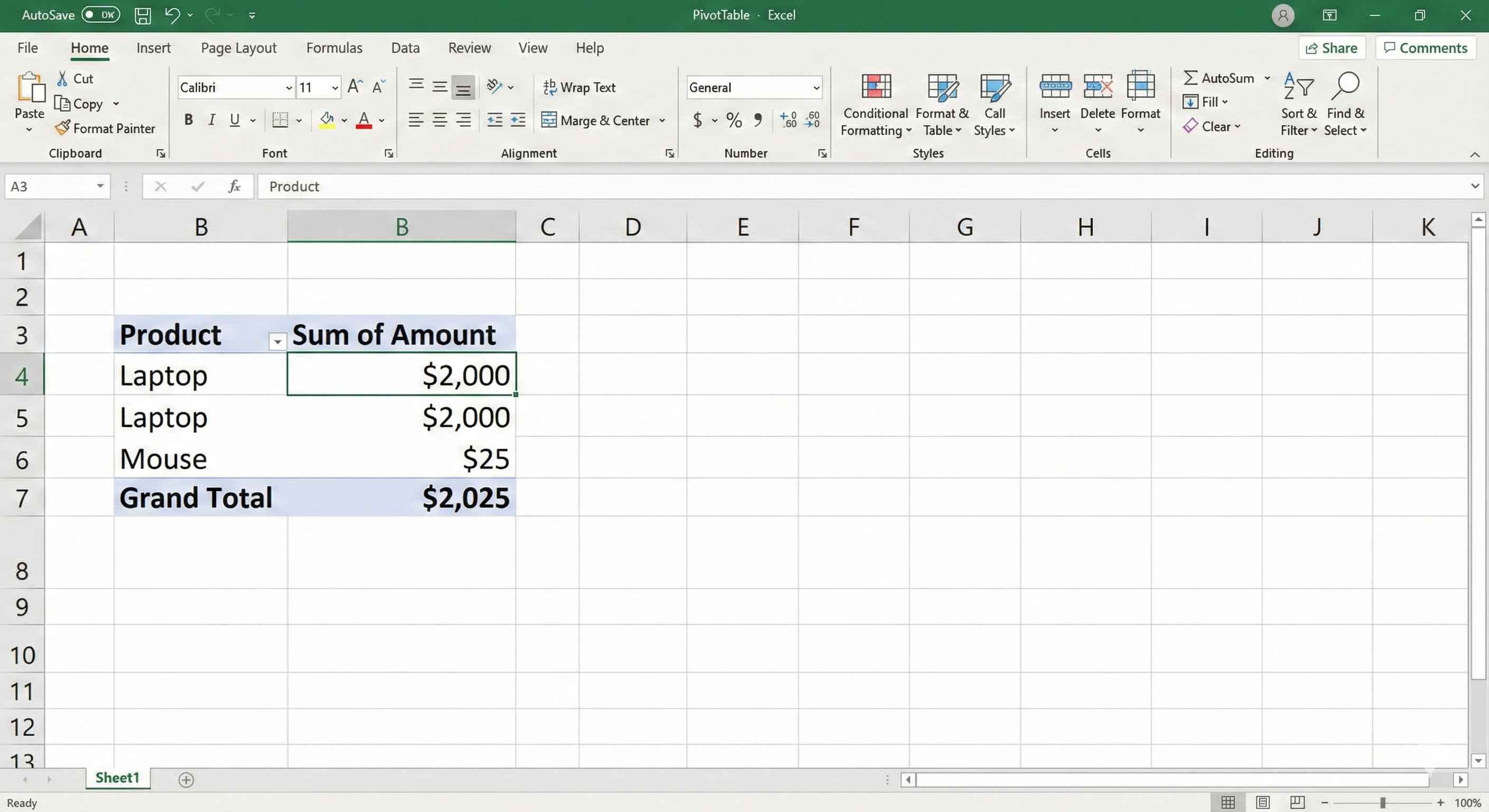
PivotTable result (instant summary):
| Product | Total Sales |
|---|---|
| Laptop | 2000 |
| Mouse | 25 |
No formulas. Just drag and drop.
How to Create a PivotTable
Step 1: Click anywhere in your data
Step 2: Go to Insert tab
Step 3: Click PivotTable
Step 4: Click OK (Excel will create it in a new sheet)
You will see a blank area on the left and a Field List on the right.

The Four Areas
When you create a PivotTable, you see four areas where you can drag fields:
| Area | What to Put Here | Example |
|---|---|---|
| Rows | Categories you want to see | Product names |
| Columns | Break down by another category | Months |
| Values | Numbers you want to add up | Sales amount |
| Filters | Filter what data to show | Region |
Example: Total Sales by Product
You have sales data. You want to see total sales for each product.
Step 1: Create PivotTable (Insert > PivotTable)
Step 2: Drag "Product" to Rows area
Step 3: Drag "Amount" to Values area
Done. You now see total sales for each product.
Example: Sales by Product and Month
You want to see sales by product, broken down by month.
Step 1: Drag "Product" to Rows
Step 2: Drag "Date" to Columns (Excel groups by month automatically)
Step 3: Drag "Amount" to Values
Now you see a table: Products down the side, Months across the top, Sales in the middle.

Changing the Calculation
By default, PivotTable adds numbers (SUM).
You can change this:
- Click on any number in the PivotTable
- Right-click > Value Field Settings
- Choose: Sum, Average, Count, Max, Min
Example: Instead of total sales, show average sale amount.
Filtering Data
You can filter to show only specific data.
Method 1: Drag a field to Filters area. A dropdown appears at the top.
Method 2: Click the dropdown arrow next to any Row or Column label.
Example: Show only sales from "East" region.
Refreshing Your PivotTable
PivotTables do NOT update automatically when you change your data.
To refresh:
- Right-click anywhere in PivotTable
- Click Refresh
Or press Alt + F5.
Common Mistakes
Mistake 1: Blank rows in your data Solution: Delete all blank rows before creating PivotTable
Mistake 2: No headers in first row Solution: Make sure row 1 has column names
Mistake 3: Forgetting to refresh Solution: Always refresh after changing source data
Tips for Better PivotTables
Tip 1: Format numbers as currency Right-click a number > Number Format > Currency
Tip 2: Show in tabular form (easier to read) Design tab > Report Layout > Show in Tabular Form
Tip 3: Remove subtotals for cleaner look Design tab > Subtotals > Do Not Show Subtotals
Summary
- PivotTables summarize large data instantly
- Insert tab > PivotTable
- Drag fields to Rows, Columns, and Values areas
- Rows = categories, Values = numbers to sum
- Right-click > Refresh when data changes
- No formulas needed
PivotTables seem complex at first, but once you understand drag-and-drop, they become the easiest way to analyze data.